I know what you’re thinking… “Excel? why would I use that? I’m a serious data analyst with SQL superpowers“.
I get it.
While it doesn’t replace databases and BI tools for regular reporting, Excel may be just what you need for quick analysis and cleansing of small data sets.
Here are 25 tips, tricks, tweaks to make it work for you.
Getting set up
Shortcuts
Formatting
Tools
Formulas and Functions
Security
Getting set up
If you’re like most people you probably don’t spend a lot of time customising your Excel experience using File > Options.
By exploring the menus here and making a few tweaks you can make your experience more ‘you’ and avoid having to make the same change manually each time you open a workbook.
1 – Hide the things you don’t need
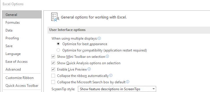
If you’d like to free up real estate by hiding away the search bar you can do so in File > Options > General.
2 – Change what happens when you press enter
You may not want the selection to move down when you press enter. To change this to right, left, or even up use the option in File > Options > Advanced.
3 – Customise the ribbon
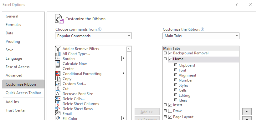
There’s no reason to keep the Ribbon as it is ‘out of the box’. Add what you need and hide what you don’t in File > Options > Customize Ribbon.
4 – Make a map
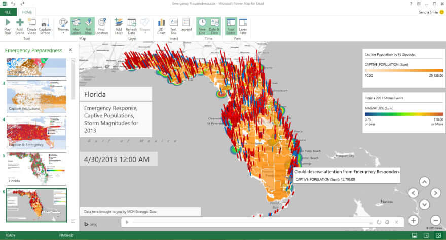
Microsoft PowerMap, and other useful add-ins, can be set up from File > Options > Customize Ribbon.
DISCLAIMER: This may not be available on all operating systems
Shortcuts
Shortcuts will save you time clicking through menus and remembering where to find what you need.
5 – One click to select all
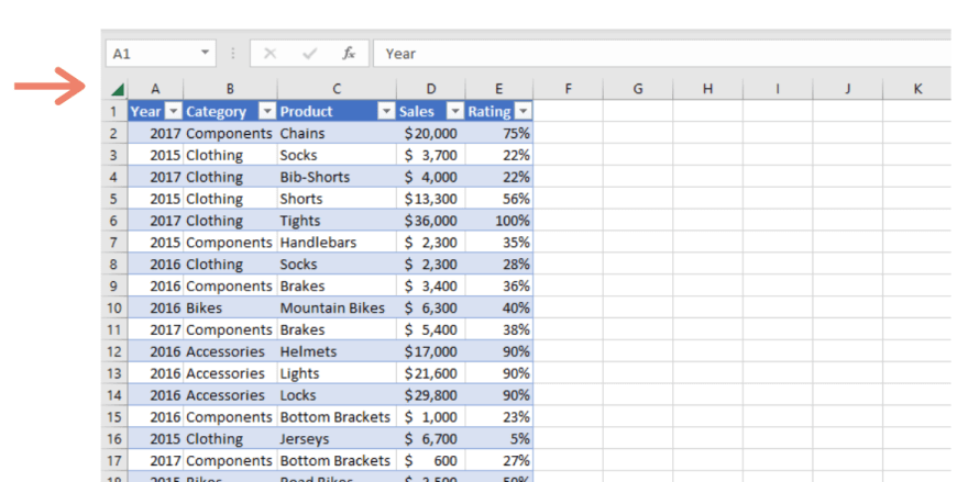
Selecting all cells is a useful way to make a change to everything in your workbook, whether that’s the cell colour, font, or adding borders to all.
This can be done by either clicking the Select All button at the top left corner or using CTL+A.
6 – Highlighting large numbers of rows
When your sheets start getting large you can spend more time than you’d like navigating around. Save time by highlighting large areas of data by using CTL+SHIFT+up/down/left/right. That way you won’t spend your day scrolling forever.
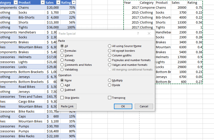
7 – Paste special
You probably know you can use CTL+C to copy, and CTL+V to paste. You may even know about the Paste Special menu. But did you know you can use keyboard shortcuts to do it all?
- Values only – Alt+E+S+V + Enter
- Formatting only – Alt+E+S+T + Enter
- Comments only – Alt+E+S+C + Enter
- Set column width same as copied cells – Alt+E+S+W + Enter
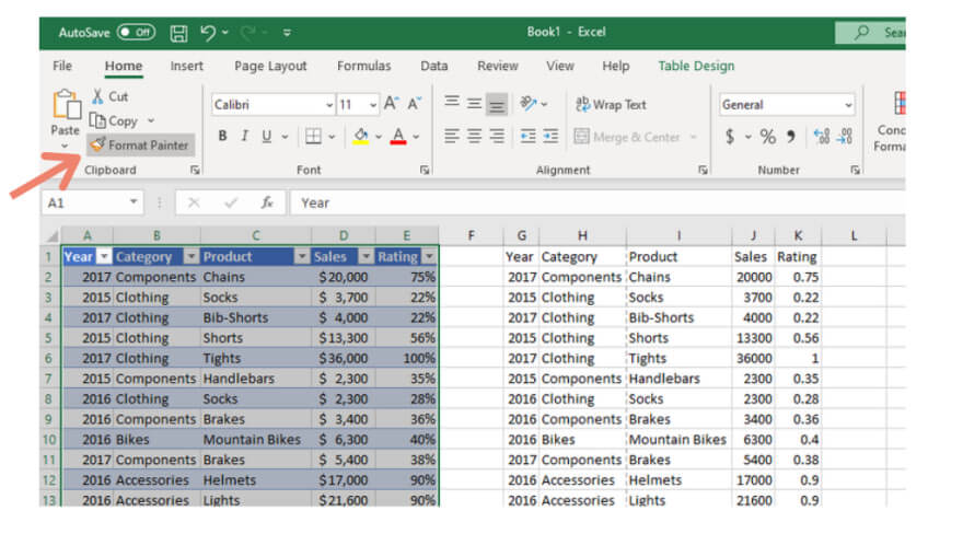
8 – Paste formatting with the paintbrush
If you like the look of a formatted area, you can quickly use the format paintbrush to apply it anywhere else you like.
Highlight the area you have in mind, click the paintbrush, then click the destination area to copy it over.
If you have multiple areas to format just double-click the paintbrush.
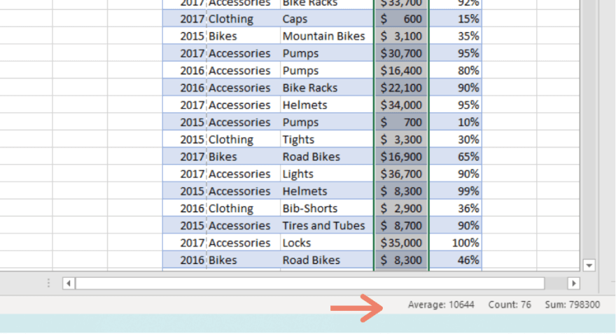
9 – Formulas without the formulas
To see SUM, COUNT, AVG super quickly, there’s no need to use formulas. Just highlight the data you need and check out the bottom right corner for the result.
10 – Fill down fast
If you have data that you need to copy down a column you can do it with a double-click. Hover in the bottom right corner of the cell until a small black cross appears, then pull down to copy down.
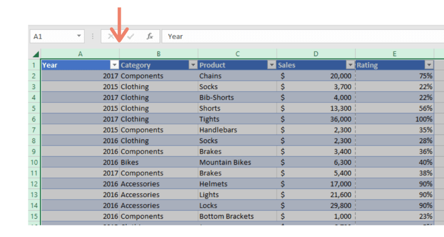
11 – Format the column to fit the text
To quickly format one or more columns to be the right width for your data, position your mouse over the right border of the column heading until the double-headed arrow appears, and then double-click the border.
12 – Add a new line to a cell
In Excel, if you hit Enter you will move to the next cell. If you’d rather have a new line in the same cell use ALT+Enter instead.
Formatting
Now it’s time for some fun with formatting. These tips make it easy to make your numbers look great.
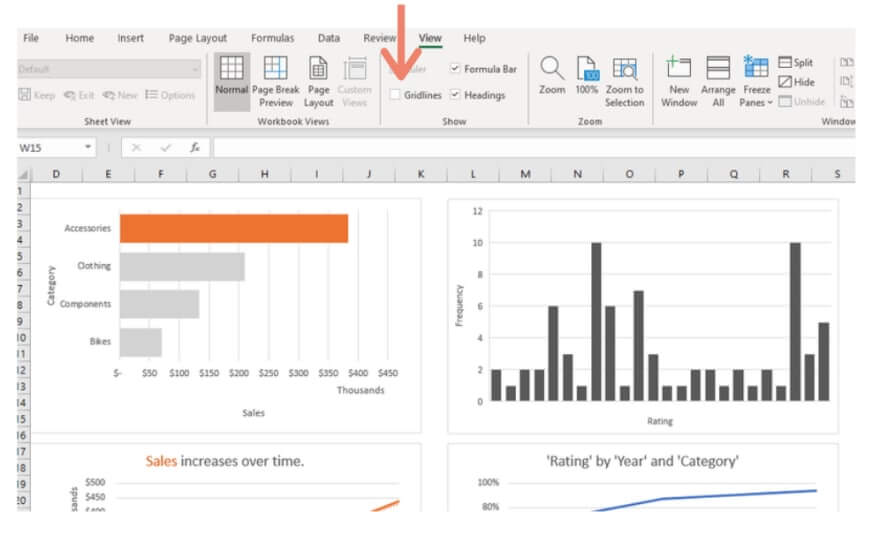
13 – Remove gridlines for cleaner dashboards
Gridlines are great when wrangling data, not so great when presenting dashboards. These can be turned off by finding the option in the View menu on the ribbon.
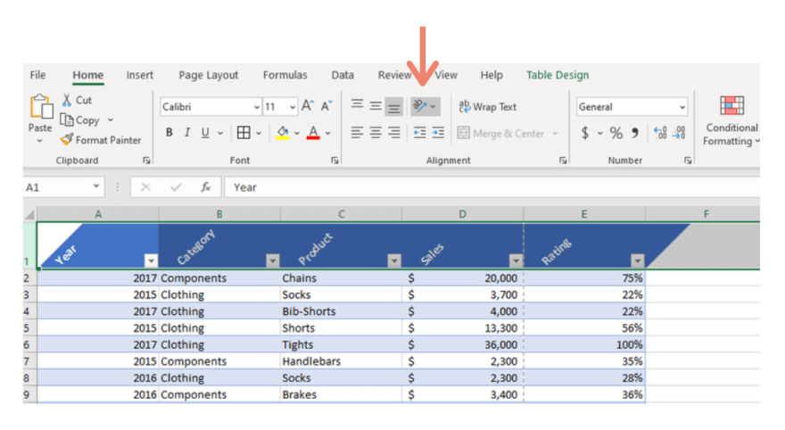
14 – Rotate headings
Headings don’t need to stay horizontal. If you have narrow columns they may look better rotated on an angle or even vertical. Find this option on the ribbon under Home > Alignment.
15 – Wrap text
While we are on the alignment menu this is also a good time to bring up the other options here. Use Wrap Text to wrap extra-long text across multiple lines.
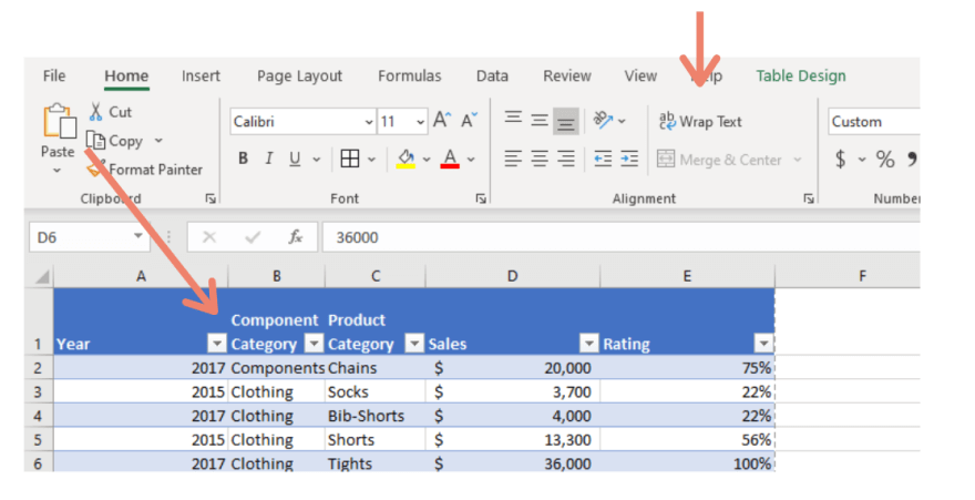
16 – Merge cells
If you have text that needs to be merged across multiple cells you can find Merge & Center here to do just that.
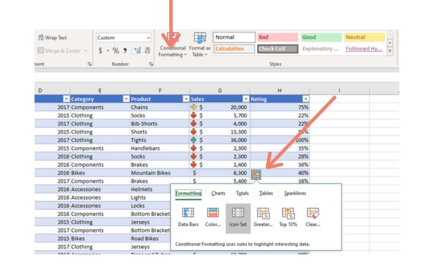
17 – Conditional formatting
The quickest way to get a feel for trends in your data is to add some conditional formatting. You can find this menu either on the Ribbon under Home > Styles or when highlighting a data set.
There’s more to it than just highlighting the top and bottom results. You can add icons, data bars, sparklines, or add some logic to make sure the right data points stand out.
Tools
18 – Split a cell in two
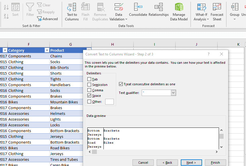
This is probably one of my favourite tools in Excel to use when cleansing data. To split a cell by a space, a symbol, a letter, or any other text qualifier use the Text to Columns tool under Data Tools.
19 – Remove duplicates
Alongside the Text to Columns tool you’ll find the Remove Duplicates tool. Highlight a column where you suspect there are duplicates and click the button to delete the duplicated data.
If you’d prefer to use a formula to do this use:
|
1 2 |
=UNIQUE(A:A) -- returns a list of distinct values from column A |
Formulas and Functions
There are hundreds of functions in Excel that can be used from anything from cleansing text to forecasting and adding complex logic.
20 – Clean up text
Cells with text can be quickly converted to the same case with the help of functions. This is especially useful when a csv or sheet of names or email addresses needs to be cleansed.
|
1 2 3 |
=UPPER(A:A) -- returns a list of UPPER case text from column A =LOWER(A:A) -- returns a list of lower case text from column A =PROPER(A:A) -- returns a list of Proper case text from column A |
21 – Trim
To further clean up text, use TRIM to remove trailing and leading spaces.
|
1 |
=TRIM(A:A) -- removes leading and trailing spaces |
22 – Concatenate quickly
To join cells together, maybe if you’ve been supplied a First Name and Last Name column and want a Full Name column, use CONCATENATE.
|
1 |
=CONCATENATE(H15, ,H16) -- concatenates H15 and H16 into one cell with a space between |
23 – Count text
You may have heard of the COUNT function which counts the number of cells in a range that contains numbers. But there are more options in this function family.
|
1 2 3 |
=COUNTA(H5:H29) -- counts the number of cells in a range which are not empty =COUNTIF(E65:E76,2015) -- counts the number of cells in a range which meet a condition, in this case =2015 |
24 – Create a countdown
Returning the system time and date is a useful function to create a countdown. Use it on a sales dashboard to countdown till the end of the month, or count down till your trip on a sheet where you track savings goals.
|
1 2 |
=TODAY() -- returns the current date =NOW() -- returns the current date and time |
Security
25 – Protect your sheet
There’s nothing worse than sending a sheet and finding someone has edited a cell in error. Prevent this by using the options in the ribbon under Review to protect cells or the whole workbook.
Excel is easy to learn and allows analysts and stakeholders to speak the same language. While it doesn’t replace databases and BI tools for regular reporting, Excel may be just what you need for quick analysis and cleansing of small data sets.
What are your most-used Excel functions and tools?
Photo by cottonbro from Pexels


Comments are closed, but trackbacks and pingbacks are open.