VLOOKUP lets Excel do the hard work of matching up a value from one spreadsheet to another. It saves time and is an essential Excel tool.
Step 1: setting up
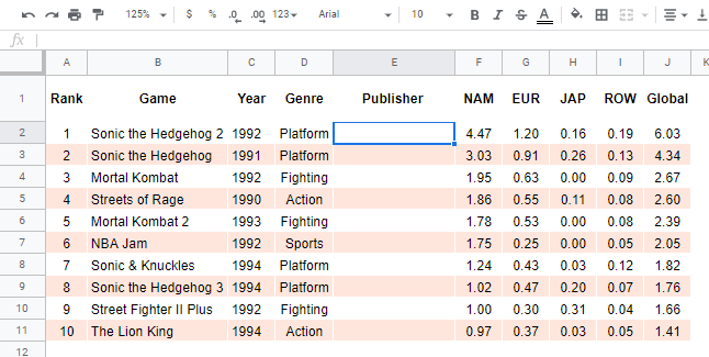
In this example, we have a sheet called games report. It has everything we need except the publisher, which we can find on the publisher report sheet.
Both sheets contain the “game” column which is what we use to match up the two sheets. The same way you would if you were trying to do this manually. This is called the reference column.
Step 2: the reference column
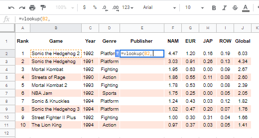
A VLOOKUP works from left to right so the column where the formula, and result, goes needs to be on the right of the reference column. Sometimes this means you may need to rearrange your data.
Type into your formula bar =VLOOKUP( and enter the first cell in the reference column.
Step 3: the table array
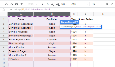
The second part of the formula is to tell the VLOOKUP where the data we want to return is.
In the example, we move to the publisher report sheet and highlight all of column A, where the reference data is. And all of column B, where the publisher data we want to return is.
Step 4: the index
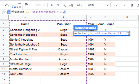
The next part of the formula is to tell the VLOOKUP how many columns from the reference column it needs to look for the data we need.
In this example the data we want is in the second column so we need to enter the number 2.
Step 5: the match
The last part of the formula is to decide if we want to return an exact match or not. To return an exact match enter a 0 and the formula is complete. If for any reason you do not want an exact match enter a 1.
To tidy things up we just need to copy the formula down and the data will follow.
Remember to copy and ‘paste values’ to ensure you the results remain and not the formula. If for any reason your lookup table moves or is deleted, so will your results.
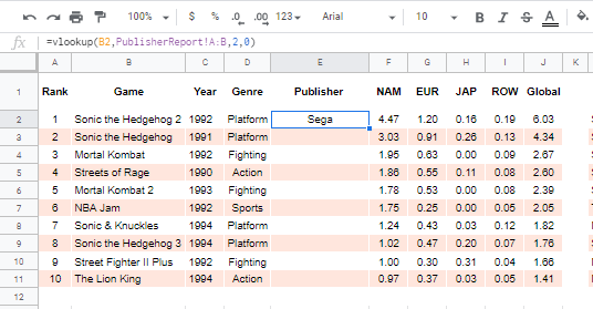
Photo by Jesús Mirón García from Pexels

